
In this project, my goal is to write a software pipeline to detect vehicles in a video.
- Perform a Histogram of Oriented Gradients (HOG) feature extraction on a labeled training set of images and train a classifier Linear SVM classifier
- Apply a color transform and append binned color features, as well as histograms of color, to my HOG feature vector.
- Implement a sliding-window technique and use my trained classifier to search for vehicles in images.
- Run the pipeline on a video stream and create a heat map of recurring detections frame by frame to reject outliers and follow detected vehicles.
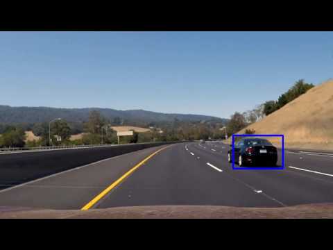
- Estimate a bounding box for vehicles detected.
git clone [email protected]:ckirksey3/vehicle-detection-with-svm.git
cd vehicle-detection-with-svm
If you don't already have tools like Jupyter and OpenCV installed, follow the Udacity instructions to configure an anaconda environment that will give you these tools.
Download and unzip the training data into a new directory called "train" within the vehicle-detection-with-svm directory.
jupyter notebook
To see the code in practice, execute each cell in succession by pressing shift + enter. You can also run the whole notebook in a single step by clicking on the menu Cell -> Run All.
I used a Linear SVM to classify image segments from the car's camera as either vehicles or non-vehicles. The key to building an accurate classifier was feeding it the right features.

A key feature in my classification process is Histogram of Oriented Gradients or HOG (this paper gives further detail). This effectively extracts the orientation of sampled edges throughout the image to give our classifier a general sense of the shape inside of the image without having to feed in the entire image. It helps our classifier generalize it's learnings to images taken from different angles or of cars with different portions.
To tune my usage of the hog feature, I began with a basic car image from the training set. I applied the hog function using the hyperparemeter values from the lesson (9 orientations, 8 pixels per cell, and 2 cells per block). Then I displayed that image in my notebook. This confirmed that the function was correctly extracting gradient features.
Next, I experimented with different values for the hyperparameters to see if I could more accurately detect the unique shape of a vehicle. I evaluated the impact of my tweaks by looking at the image produced by the hog function and the impact that the tweak had on my SVL classifier's overall accuracy.
Ultimately I found that using YCrCB color space, 9 orientations, 8 pixels per cell, and 2 cells per block were very effective. One change that I made was using all of the hog channels and increase of my spatial and color histogram bins. These modifications made my overall pipeline significantly slower, but improved my classification accuracy on the validation set from .96 to .99. It also improved the accuracy on my manually labeled set of windows (pulled from the project video) from .4 to .55.

Another feature that I feed to my classifier is a histogram that captures the general distribution of colors within the image, irrespective of the actual location of the colors within the image. This is very useful as many cars have similar color distributions while still having significant differences in shape.

I pulled out the spatial features of the image by feeding a downgraded (32, 32) version of each training image in RGB color space. This helps our classifier get a sense for where the different colors are within the image.

I created a set of windows that comprise a simple grid when stiched together. Then I drew those windows onto an image to confirm that they were being created correctly. Next I limited the grid to the area of the image that comprised the road.
The simple grid had the issue that in some windows the car was too small and in others the window only captured a small portion of the car. This resulted in lots of false negatives from my classifier so I implemented a process for increasing the size of the windows on every iteration of the y axis. This ensured that my window frames were larger for sections of the road that were close to the camera. After several round of tweaking the initial image size and grow rate, I was able to get windows drawn on my sample image that effectively framed the car
After finishing the rest of the pipeline and implementing a heatmap to reduce false positives, I found that simply increasing the overlap percentage was not getting me the adequate multiple confirmations for the cars to stand out from the false positives. Heavy overlap was also computationally expensive and slowed my video processing down significantly. I decided to implement a second round of window creation where I initialized the window with a slightly smaller value. This was very effective in getting confirmation from my classifier of identified cars while not increasing the rate of false positives. This window technique, combined with the heatmap thresholding, helped me get a working process.

Ultimately I searched on three different scales using RGB 3-channel HOG features plus spatially binned color and histograms of color in the feature vector. Moving to three scales improved the frequency with which my classifier saw a car image scaled similarly to its training data. It also allowed me to get multiple confirmations of the vehicle so that I could make my heatmap threshold higher and filter out more false positives.

In order to reduce false positives and draw tighter bounding boxes, I store a heatmap that persists between frames of the video in which the classification of different regions of the main image is persisted. It took some tweaking to get the heatmap to remove history from previous frames at an appropriate rate. Eventually I discovered that adding heat to the map linearly and removing it exponentially accurately found cars without leaving "ghost detections" once the car moved to a different location within the frame.

One of the key limitations to my project currently is how long the pipeline takes to process a video stream. An obvious improvement would be to precompute HOG values for the image before splitting into the windows. After spending a few days working on that issue, I decided to delay it until a later iteration of the project. In its current state, the pipeline would not be useful for doing on-the-fly obstacle identification.
Another limitation is that it often fails to identify cars that are far away. In order to improve the long range accuracy of the project, I could create a more dynamic window scaling tool that samples only from areas within the road. Finally, I would still like to get tighter bounding boxes on the vehicles themselves. This could be solved by acquiring a training image set with more partial vehicle images so that I could use smaller windows.